Proposer’s Cookbook: Planning for SALT

This page provides practical examples for using saltshaker to prepare and optimize observing strategies for the Southern African Large Telescope (SALT).

Important

Essential Usage Information: saltshaker is an independent pre-planning tool and is not an official SALT product. While it provides high-fidelity models, all final observing proposals must be validated and submitted using the official SALT Phase I Proposal Tool (PIPT).

Use these examples to screen targets, optimize your strategy, and generate preliminary plots for your Technical Justification, but always perform a final check in the PIPT before submission.

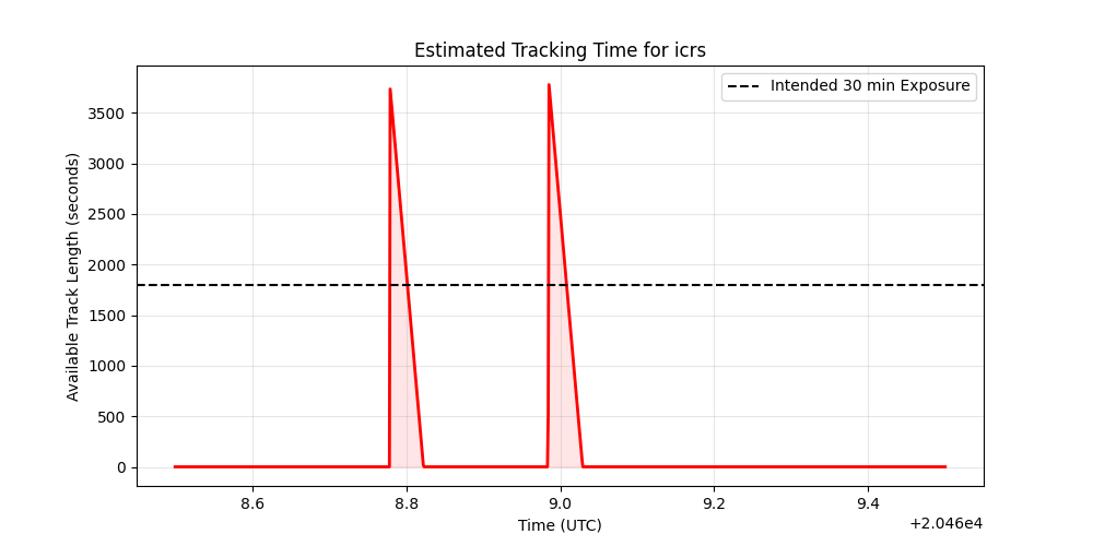
Preliminary Feasibility: Estimating Track Lengths

The most fundamental constraint at SALT is the tracker’s physical range. For any exposure, you should verify that the telescope can follow the target for the required duration.

The following plot can help you estimate the available “window of opportunity” for your intended exposures during the proposal phase.

import numpy as np
import matplotlib.pyplot as plt
from astropy.coordinates import SkyCoord
from astropy.time import Time
import astropy.units as u
from saltshaker import get_track_length

# Define your target and the night of interest
target = SkyCoord.from_name('Sirius')
obs_date = '2026-01-15'
start_time = Time(f"{obs_date} 12:00:00")

# Sample the tracking zone over 24 hours
times = start_time + np.linspace(0, 24, 1000) * u.hour
track_lengths = [get_track_length(target, t).to(u.second).value for t in times]

plt.figure(figsize=(10, 5))
plt.fill_between(times.plot_date, track_lengths, color='red', alpha=0.1)
plt.plot(times.plot_date, track_lengths, color='red', lw=2)

# Reference line for an intended 30-minute exposure
plt.axhline(1800, color='black', linestyle='--', label='Intended 30 min Exposure')

plt.title(f"Estimated Tracking Time for {target.name}")
plt.ylabel("Available Track Length (seconds)")
plt.xlabel("Time (UTC)")
plt.legend()
plt.grid(True, alpha=0.3)
plt.show()

(Source code, png, pdf)

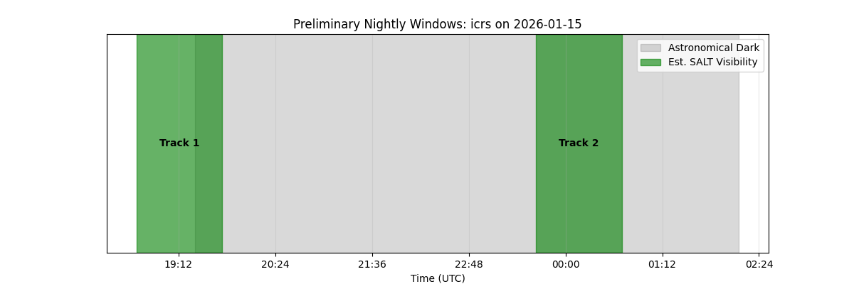
Nightly Planning: Visualizing Preliminary Tracks

Because SALT is a fixed-altitude telescope, targets often pass through the visibility zone twice (the East and West tracks), separated by a “Zenith Hole.”

This visualization helps you understand when your target is observable relative to astronomical twilight (-18°).

from saltshaker import get_visibility_windows, get_salt_observer
from astropy.coordinates import SkyCoord
from astropy.time import Time
import astropy.units as u
import matplotlib.pyplot as plt
from matplotlib.dates import DateFormatter

observer = get_salt_observer()
target = SkyCoord.from_name('Sirius')
date = '2026-01-15'

# 1. Calculate the estimated tracks and twilight
windows = get_visibility_windows(target, date)
start_time = Time(f"{date} 12:00:00")
eve_twi = observer.twilight_evening_astronomical(start_time, which='next')
morn_twi = observer.twilight_morning_astronomical(eve_twi, which='next')

# 2. Create the visualization
fig, ax = plt.subplots(figsize=(12, 4))

# Shade the dark time
ax.axvspan(eve_twi.plot_date, morn_twi.plot_date, color='black', alpha=0.15, label='Astronomical Dark')

# Shade the estimated visibility windows
for i, w in enumerate(windows):
    ax.axvspan(w.start_time.plot_date, w.end_time.plot_date, color='green', alpha=0.6,
               label='Est. SALT Visibility' if i==0 else "")
    # Label the tracks
    mid_time = w.start_time.plot_date + (w.end_time.plot_date - w.start_time.plot_date)/2
    ax.text(mid_time, 0.5, f"Track {i+1}", ha='center', va='center', fontweight='bold')

plt.title(f"Preliminary Nightly Windows: {target.name} on {date}")
ax.xaxis.set_major_formatter(DateFormatter('%H:%M'))
ax.set_yticks([])
plt.xlabel("Time (UTC)")
plt.legend(loc='upper right')
plt.grid(True, axis='x', alpha=0.3)
plt.show()

(Source code, png, pdf)

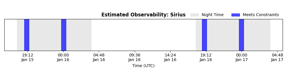
Preliminary Scheduling: Moon and Track Length

Using saltshaker with astroplan allows you to estimate when your target meets both SALT’s tracking requirements and your project’s preliminary lunar constraints. This visualization includes environmental context (night/day) to help you understand the specific observing windows.

import numpy as np
import matplotlib.pyplot as plt
import matplotlib.dates as mdates
import astropy.units as u
from astropy.coordinates import SkyCoord
from astropy.time import Time
from astroplan import FixedTarget, is_event_observable
from saltshaker import (
    get_salt_observer,
    SaltTrackLengthConstraint,
    SaltMoonConstraint
)

# 1. Setup the Observer and Target
observer = get_salt_observer()
target = FixedTarget(coord=SkyCoord.from_name('Sirius'), name='Sirius')

# 2. Define Constraints (e.g., Gray moon and minimum 20 min track)
constraints = [
    SaltTrackLengthConstraint(min_track_length=20 * u.minute),
    SaltMoonConstraint(max_illumination=0.5)
]

# 3. Evaluate over a 48-hour period
start_time = Time('2026-01-15 12:00:00')
times = start_time + np.linspace(0, 48, 300) * u.hour

# 4. Calculate observability and night/day states
observable = is_event_observable(constraints, observer, target, times=times)[0]
is_night = observer.is_night(times)

# 5. Visualize the Timeline
fig, ax = plt.subplots(figsize=(10, 2.5))

# Shade the Night Time (in light grey)
ax.fill_between(times.plot_date, 0, 1, where=is_night,
                color='lightgrey', alpha=0.5, label='Night Time')

# Shade the Observability Window (in blue)
ax.fill_between(times.plot_date, 0, 1, where=observable,
                color='blue', alpha=0.7, label='Meets Constraints')

# Formatting the plot
ax.set_yticks([])
ax.set_ylim(0, 1)
ax.xaxis.set_major_formatter(mdates.DateFormatter('%H:%M\n%b %d'))

plt.title(f"Estimated Observability: {target.name}", fontsize=12, fontweight='bold')
plt.xlabel("Time (UTC)")
plt.legend(loc='upper right', bbox_to_anchor=(1, 1.3), ncol=2, frameon=False)
plt.tight_layout()
plt.show()

(Source code, png, pdf)

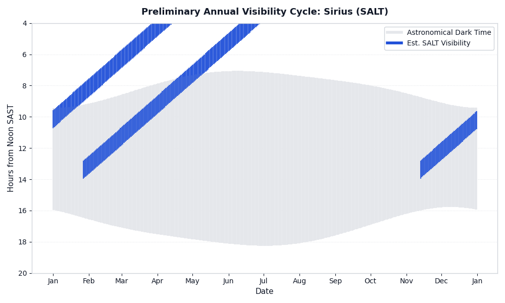
Long-term Planning: Annual Visibility Cycles

The “Annual Plot” provides a rough guide for when your target is best placed during the semester. This visualization uses a daily sampling rate to create a smooth “carpet” effect, showing how visibility windows shift across the night as the Earth orbits the Sun.

import numpy as np
import matplotlib.pyplot as plt
import matplotlib.dates as mdates
from matplotlib.lines import Line2D
from astropy.coordinates import SkyCoord
from astropy.time import Time
import astropy.units as u
from saltshaker import get_salt_observer, get_visibility_windows

# --- Configuration & Setup ---
target_name = 'Sirius'
year = 2026

observer = get_salt_observer()
target = SkyCoord.from_name(target_name)

# Sample every 1 day for a smooth, continuous "carpet" effect
dates = Time(f"{year}-01-01") + np.arange(0, 365, 1) * u.day

# --- Color Palette (Clean Documentation) ---
BG_COLOR = '#FFFFFF'        # Pure white background
NIGHT_COLOR = '#E5E7EB'     # Soft light-grey for dark time
TRACK_COLOR = '#1D4ED8'     # Bold, high-contrast blue for visibility tracks
TEXT_COLOR = '#111827'      # Near-black for crisp, legible text
GRID_COLOR = '#D1D5DB'      # Subtle grey for gridlines

# --- Plotting ---
plt.figure(figsize=(10, 6))

for date in dates:
    windows = get_visibility_windows(target, date)
    try:
        # Calculate twilight limits
        eve = observer.twilight_evening_astronomical(date, which='next')
        morn = observer.twilight_morning_astronomical(eve, which='next')

        # Base time: 10:00 UTC (12:00 SAST) to keep the night continuous
        base = Time(f"{date.iso.split()[0]} 10:00:00")
        to_h = lambda t: (t - base).to(u.hour).value

        # Plot Dark Time as vertical slices
        plt.plot([date.datetime, date.datetime], [to_h(eve), to_h(morn)],
                 color=NIGHT_COLOR, alpha=1.0, lw=2)

        # Plot SALT Visibility Tracks
        for w in windows:
            plt.plot([date.datetime, date.datetime], [to_h(w.start_time), to_h(w.end_time)],
                     color=TRACK_COLOR, lw=2, alpha=0.9)
    except Exception:
        continue

# --- Formatting & Styling ---
ax = plt.gca()
ax.set_facecolor(BG_COLOR)
plt.gcf().patch.set_facecolor(BG_COLOR)

# Titles and Labels
plt.title(f"Preliminary Annual Visibility Cycle: {target_name} (SALT)",
          color=TEXT_COLOR, fontsize=13, pad=12, fontweight='bold')
plt.xlabel("Date", color=TEXT_COLOR, fontsize=11, fontweight='500')
plt.ylabel("Hours from Noon SAST", color=TEXT_COLOR, fontsize=11, fontweight='500')

# Axis Ticks and Spines styling
ax.xaxis.set_major_locator(mdates.MonthLocator())
ax.xaxis.set_major_formatter(mdates.DateFormatter('%b'))
ax.tick_params(colors=TEXT_COLOR, which='both', labelsize=10)

for spine in ax.spines.values():
    spine.set_color(GRID_COLOR)
    spine.set_linewidth(1)

# Grid and limits
plt.grid(True, axis='y', alpha=0.6, color=GRID_COLOR, linestyle=':')
ax.set_ylim(4, 20)
ax.invert_yaxis()

# Custom Legend
custom_lines = [
    Line2D([0], [0], color=NIGHT_COLOR, lw=4),
    Line2D([0], [0], color=TRACK_COLOR, lw=4)
]
legend = plt.legend(custom_lines, ['Astronomical Dark Time', 'Est. SALT Visibility'],
                    loc='upper right', framealpha=1.0,
                    facecolor=BG_COLOR, edgecolor=GRID_COLOR, fontsize=10)
for text in legend.get_texts():
    text.set_color(TEXT_COLOR)

plt.tight_layout()
plt.show()

(Source code, png, pdf)

Semester Statistics: Guiding Time Requests

Calculating preliminary statistics on observable hours helps you determine if your project is realistic for a given semester.

import astropy.units as u
from astropy.coordinates import SkyCoord
from saltshaker import get_visibility_windows, get_semester_nights

target = SkyCoord.from_name('NGC 300')
year, semester = 2026, 1
nights = get_semester_nights(year, semester)

total_sec = 0
observable_nights = 0

for eve, morn in nights:
    windows = get_visibility_windows(target, eve)
    night_sec = 0
    for w in windows:
        # Estimate overlap of the SALT track with dark time
        start = max(w.start_time, eve)
        end = min(w.end_time, morn)
        if start < end:
            night_sec += (end - start).to(u.second).value

    if night_sec > 0:
        total_sec += night_sec
        observable_nights += 1

print(f"Preliminary Statistics for {target.name} (Semester {year}-{semester}):")
print(f"  - Estimated Total Observable Hours: {total_sec / 3600:.1f} hours")
print(f"  - Number of Observable Nights: {observable_nights}")
print(f"  - Estimated Average Track per Night: {(total_sec/observable_nights)/60:.1f} minutes")

Example Output:

Preliminary Statistics for NGC 300 (Semester 2026-1):
  - Estimated Total Observable Hours: 161.3 hours
  - Number of Observable Nights: 132
  - Estimated Average Track per Night: 73.3 minutes

Catalog Screening: Preliminary Catalog Feasibility

If your project involves a large catalog of targets, you can use these functions to quickly screen for objects that fall within SALT’sreachable range.

import pandas as pd
from astropy.coordinates import SkyCoord
from saltshaker import is_target_observable

# Preliminary target catalog
catalog = [
    ('M31', '00h42m44s', '+41d16m09s'),
    ('M42', '05h35m17s', '-05d23m28s'),
    ('Omega Cen', '13h26m47s', '-47d28m46s'),
    ('Centaurus A', '13h25m27s', '-43d01m08s'),
]

results = []
for name, ra, dec in catalog:
    coord = SkyCoord(ra, dec, frame='icrs')
    # is_target_observable provides a quick preliminary check
    observable = is_target_observable(coord)
    results.append({'Target': name, 'Dec': dec, 'Est. SALT Observable': observable})

df = pd.DataFrame(results)
print(df.to_string(index=False))

Example Output:

     Target         Dec  Est. SALT Observable
        M31  +41d16m09s                 False
        M42  -05d23m28s                  True
  Omega Cen  -47d28m46s                  True
Centaurus A  -43d01m08s                  True